---
title: "simulateData_lavaan"
output: html_document
date: "2023-03-22"
---
```{r setup, include=FALSE}
knitr::opts_chunk$set(echo = TRUE)
```
First part of this SEM exercise introduces data simulation for both singe and multi-group analysis. Second, an example of multi-group analysis is given (including measurement invariance testing across groups).
## Simulate SEM data based on previous research
We will create a simulation data based on the previous SEM exercise results with *simstandard* package.
First, let's define the model we are going to use. Details are available in [SEM_R.Rmd](SEM_R.Rmd) and [SEM_R.html](SEM_R.html).
We will use the *marker variable method* (for other scaling options, see Beaujean, 2014, pp. 41) to scale the latent variables: One indicator (manifest) variable's loading for each latent variable is constrained to an arbitrary value (usually 1).
```{r define SEM model, warning = F, message = F}
library(lavaan)
sem_model <- '
# Factors
ENC =~ NA*v5 + v7 + 1*v17 # Encouraging leadership
BUI =~ 1*v42r + v43 # Build-up of work requirements
PSY =~ 1*v44 + v45 # Psychic stress of the work
# Regressions
PSY ~ ENC + BUI # Predict PSY with ENC and BUI
# Covariances
ENC ~~ BUI # Let ENC and BUI correlate
'
```
Second, we need to fit the model:
```{r fit SEm model, warning = F, message = F}
# read in dfttu4 data (n = 447)
dfttu4 <- read.csv("data1_csv.dat", header = T)
sem_model_fit <- sem(sem_model,
data=dfttu4,
mimic="mplus",
group = NULL, # no grouping variable (e.g., gender, control/intervention,...)
cluster = NULL, # no clustering variable (e.g., multilevel data may contain several values for each participant)
missing = "fiml.x" # full information maximum likelihood approach
)
```
Is our model under/just/overidentified?
```{r number of parameters, warning = F, message = F}
# how many parameters are to be estimated in the model?
inspect(sem_model_fit) # 24
# the model is overidentified (good!) as there are 28 non-redundant elements [7(7+1)/2 = 56/2 = 28]
# and 24 parameters to be estimated (28 - 24 = 4):
#
# 4 manifest variable loadings on three factors (lambda matrix)
# 7 error variances of manifest variables (theta matrix)
# 3 latent variances and 1 covariance (psi matrix)
# 2 regressions (beta matrix)
# 7 intercepts(nu matrix)
```
We may proceed as the model is overidentified.
Third, we'll check the results.
Note that "Estimate" column reports unstandardized values, while "Std.lv" column reports values when latent variables are standardized and "Std.all" column values reflect situation when both latent and observed (manifest) values are standardized.
```{r SEM results, warning = F, message = F}
summary(sem_model_fit,
standardized=TRUE,
rsq=TRUE,
fit.measures = T)
# Latent Variables:
# Estimate Std.Err z-value P(>|z|) Std.lv Std.all
# ENC =~
# v5 0.896 0.048 18.766 0.000 0.962 0.814
# v7 0.765 0.043 17.629 0.000 0.822 0.768
# v17 1.000 1.074 0.886
# BUI =~
# v42r 1.000 0.777 0.672
# v43 0.798 0.089 8.924 0.000 0.620 0.571
# PSY =~
# v44 1.000 1.118 0.901
# v45 0.592 0.068 8.702 0.000 0.662 0.551
#
# Regressions:
# Estimate Std.Err z-value P(>|z|) Std.lv Std.all
# PSY ~
# ENC -0.104 0.063 -1.653 0.098 -0.100 -0.100
# BUI 1.223 0.152 8.028 0.000 0.850 0.850
#
# Covariances:
# Estimate Std.Err z-value P(>|z|) Std.lv Std.all
# ENC ~~
# BUI -0.253 0.062 -4.092 0.000 -0.303 -0.303
# Variances:
# Estimate Std.Err z-value P(>|z|) Std.lv Std.all
# .v5 0.473 0.047 9.978 0.000 0.473 0.338
# .v7 0.470 0.041 11.380 0.000 0.470 0.410
# .v17 0.317 0.048 6.588 0.000 0.317 0.216
# .v42r 0.736 0.080 9.226 0.000 0.736 0.549
# .v43 0.795 0.067 11.829 0.000 0.795 0.674
# .v44 0.291 0.119 2.458 0.014 0.291 0.189
# .v45 1.002 0.079 12.747 0.000 1.002 0.696
# ENC 1.153 0.105 10.934 0.000 1.000 1.000
# BUI 0.604 0.098 6.186 0.000 1.000 1.000
# .PSY 0.269 0.132 2.035 0.042 0.215 0.215
```
There is also a third type of standardization ("Std.nox") where variables are standardized except for the exogenous observed (manifest) variables:
```{r add Std.nox, warning = F, message = F}
head(parameterEstimates(sem_model_fit, standardized = T, ci = F))
# lhs op rhs est se z pvalue std.lv std.all std.nox
# 1 ENC =~ v5 0.896 0.048 18.766 0 0.962 0.814 0.814
# 2 ENC =~ v7 0.765 0.043 17.629 0 0.822 0.768 0.768
# 3 ENC =~ v17 1.000 0.000 NA NA 1.074 0.886 0.886
# 4 BUI =~ v42r 1.000 0.000 NA NA 0.777 0.672 0.672
# 5 BUI =~ v43 0.798 0.089 8.924 0 0.620 0.571 0.571
# 6 PSY =~ v44 1.000 0.000 NA NA 1.118 0.901 0.901
```
This is the figure based on standardized results:
```{r plot SEM figure, warning = F, message = F}
library(semPlot)
semPlot::semPaths(sem_model_fit,
layout="tree",
"std", # display standardized parameter estimates
edge.label.cex=0.7,
edge.width=0.2,
edge.color="black",
optimizeLatRes=TRUE,
label.scale=TRUE,
normalize=TRUE,
fade=FALSE,
# filetype = "jpg", # save file
# filename = "SEM_figure",
as.expression=c("nodes"))
```
```{r simulate data based on SEM results above with simstandard::sim_standardized, warning = F, message = F}
library(lavaan)
# we'll use the same syntax than before, but upgraded with estimates taken from the results of the earlier SEM model (above)
sem_model_simulation <- '
# Factors
ENC =~ 0.81*v5 + 0.77*v7 + 0.87*v17 # standardized loadings from "Std.all" output above
BUI =~ 0.67*v42r + 0.57*v43
PSY =~ 0.90*v44 + 0.55*v45
# Regressions
PSY ~ -0.10*ENC + 0.85*BUI # standardized path coefficients from "Std.all" output above
# Covariances
ENC ~~ -.30*BUI # covariance from "Std.all" output above
'
# install.packages("simstandard")
library(simstandard)
# simulate data
set.seed(2023)
simulated_data <- simstandard::sim_standardized(sem_model_simulation, n = 100000)
```
```{r look at matrices, warning = F, message = F}
# Schneider's tutorial
# https://cran.r-project.org/web/packages/simstandard/vignettes/simstandard_tutorial.html
# has a really nice "ggcor" function to display matrices:
ggcor <- function(d) {
require(ggplot2)
as.data.frame(d) %>%
tibble::rownames_to_column("rowname") %>%
tidyr::pivot_longer(-rowname, names_to = "colname", values_to = "r") %>%
dplyr::mutate(rowname = forcats::fct_inorder(rowname) %>% forcats::fct_rev()) %>%
dplyr::mutate(colname = factor(colname,
levels = rev(levels(rowname)))) %>%
ggplot(aes(colname, rowname, fill = r)) +
geom_tile(color = "lightgray") +
geom_text(aes(label = formatC(r, digits = 2, format = "f") %>%
stringr::str_replace_all("0\\.",".") %>%
stringr::str_replace_all("1.00","1")),
color = "white",
fontface = "bold",
family = "serif") +
scale_fill_gradient2(NULL,
na.value = "darkgrey",
limits = c(-1.01, 1.01),
high = "darkred",
low = "darkblue") +
coord_equal() +
scale_x_discrete(NULL,position = "top") +
scale_y_discrete(NULL) +
theme_light(base_family = "serif", base_size = 12) +
theme(axis.text.x = element_text(angle = 90))
}
# check covariances
# cov(simulated_data) # quite good match with the original results!
# a way lot easier to read
cov(simulated_data) %>% ggcor() +
labs(title="covariance matrix of the observed and latent variables")
# inspect the matrices (A, S) that simstandard uses to create the data
sem_model_simulation_matrices <- sim_standardized_matrices(sem_model_simulation)
# Reticular Action Model (RAM) by McArdle (1978)
# See Ferrer et al. (2019, pp. 126-142) chapter
#
# A matrix contains all the asymmetric path coefficients (i.e., the loadings and the structural coefficients).
sem_model_simulation_matrices$RAM_matrices$A %>% ggcor() +
labs(title="A matrix: loadings and the structural coefficients")
# S matrix contains all the symmetric path coefficients (i.e., the variances and correlations of the observed and latent variables)
sem_model_simulation_matrices$RAM_matrices$S %>% ggcor() +
labs(title="S matrix: variances and correlations of the observed \n and latent variables")
```
We can see that the simulated data is close to the "sem_model_simulation" with fixed parameters:
```{r, warning = F, message = F}
# ENC =~ 0.81*v5 + 0.77*v7 + 0.87*v17
# BUI =~ 0.67*v42r + 0.57*v43
# PSY =~ 0.90*v44 + 0.55*v45
#
# PSY ~ -0.10*ENC + 0.85*BUI
#
# ENC ~~ -.30*BUI
```
Next, we'll see how the *lavaan* output with simulated data and non-fixed model compares to the simulation results.
```{r verify simulated data with lavaan output, warning = F, message = F}
# # this was the original "sem_model_simulation" model:
# #
# sem_model_simulation <- '
#
# # Factors
# ENC =~ 0.81*v5 + 0.77*v7 + 0.87*v17 # standardized loadings from "Std.all" output above
# BUI =~ 0.67*v42r + 0.57*v43
# PSY =~ 0.90*v44 + 0.55*v45
#
# # Regressions
# PSY ~ -0.10*ENC + 0.85*BUI # standardized path coefficients from "Std.all" output above
#
# # Covariances
# ENC ~~ -.30*BUI # covariance from "Std.all" output above
# '
# we'll make a new version of model where all fixed parameters are set free
sem_model_simulation_free <- simstandard::fixed2free(sem_model_simulation)
# # check
# cat(sem_model_simulation_free)
# ENC ~~ BUI
# PSY ~ ENC + BUI
# BUI =~ v42r + v43
# ENC =~ v5 + v7 + v17
# PSY =~ v44 + v45
# actually, the resulting model is identical to our original model:
# sem_model <- '
# # Factors
# ENC =~ NA*v5 + v7 + 1*v17 # Encouraging leadership
# BUI =~ 1*v42r + v43 # Build-up of work requirements
# PSY =~ 1*v44 + v45 # Psychic stress of the work
# # Regressions
# PSY ~ ENC + BUI # Predict PSY with ENC and BUI
# # Covariances
# ENC ~~ BUI # Let ENC and BUI correlate
# '
# we'll use lavaan to see if the observed data in "sem_model_simulation" conform to the model in "sem_model_simulation_free"
# create simulated data
set.seed(2023)
simulated_data2 <- simstandard::sim_standardized(sem_model_simulation, # or use "sem_model"
latent = F, # Note: only following vars are included: "v5", "v7", "v17", "v42r", "v43", "v44", "v45"
errors = F,
n = 100000)
# evaluate the fit of free model on simulated data
lavaan_fit1 <- sem(model = sem_model_simulation_free,
data = simulated_data2)
# see the results
summary(lavaan_fit1,
standardized = T,
fit.measures = T)
```
```{r compare lavaan output to A and S matrices, warning = F, message = F}
# extract RAM paths
sem_model_simulation_free_matrices <- simstandard::lav2ram(lavaan_fit1)
# display asymmetric paths (i.e., single-headed arrows for loadings and structure coefficients)
sem_model_simulation_free_matrices$A %>% ggcor() +
labs(title="A matrix: loadings and the structural coefficients")
# display symmetric paths (i.e., curved double-headed arrows exogenous variances, error variances, disturbance variances, and any covariances among these)
sem_model_simulation_free_matrices$S %>% ggcor() +
labs(title="S matrix: variances and correlations of the observed \n and latent variables")
```
*lavaan* results with the simulation data match the results of model with fixed parameters:
```{r, warning = F, message = F}
# ENC =~ 0.81*v5 + 0.77*v7 + 0.87*v17
# BUI =~ 0.67*v42r + 0.57*v43
# PSY =~ 0.90*v44 + 0.55*v45
#
# PSY ~ -0.10*ENC + 0.85*BUI
#
# ENC ~~ -.30*BUI
```
So, we are happy!
Next, let's look how *lavaan::simulateData* can produce simulated data.
```{r non-grouping simulation with lavaan::simulateData, warning = F, message = F}
library(lavaan)
# compare to simstandard::sim_standardized
# define simulated measurement model (same as before)
sem_model_simulation <- '
# Factors
ENC =~ 0.81*v5 + 0.77*v7 + 0.87*v17 # standardized loadings from "Std.all" output above
BUI =~ 0.67*v42r + 0.57*v43
PSY =~ 0.90*v44 + 0.55*v45
# Regressions
PSY ~ -0.10*ENC + 0.85*BUI # standardized path coefficients from "Std.all" output above
# Covariances
ENC ~~ -.30*BUI # covariance from "Std.all" output above
'
# simulate 100 data frame rows
set.seed(2013)
simData_lavaan <- lavaan::simulateData(
sem_model_simulation,
standardized = T, # known issue to produce variances exceeding 2 if set to TRUE
# see https://github.com/yrosseel/lavaan/issues/46
sample.nobs=1000000
)
nrow(simData_lavaan)
# define measurement model
sem_model <- '
# Factors
ENC =~ NA*v5 + v7 + 1*v17 # Encouraging leadership
BUI =~ 1*v42r + v43 # Build-up of work requirements
PSY =~ 1*v44 + v45 # Psychic stress of the work
# Regressions
PSY ~ ENC + BUI # Predict PSY with ENC and BUI
# Covariances
ENC ~~ BUI # Let ENC and BUI correlate
'
# fit the model on simulated data
lavaan_fit2 <- sem(sem_model, data=simData_lavaan)
# print the summary
summary(lavaan_fit2, standardized = T, fit.measures = T)
# Latent Variables:
# Estimate Std.Err z-value P(>|z|) Std.lv Std.all
# ENC =~
# v5 0.930 0.001 852.061 0.000 0.810 0.810
# v7 0.885 0.001 817.830 0.000 0.771 0.771
# v17 1.000 0.871 0.871
# BUI =~
# v42r 1.000 0.668 0.669
# v43 0.853 0.002 439.447 0.000 0.570 0.570
# PSY =~
# v44 1.000 0.899 0.900
# v45 0.611 0.001 431.722 0.000 0.549 0.549
#
# Regressions:
# Estimate Std.Err z-value P(>|z|) Std.lv Std.all
# PSY ~
# ENC -0.103 0.001 -80.620 0.000 -0.099 -0.099
# BUI 1.145 0.003 392.682 0.000 0.851 0.851
#
# Covariances:
# Estimate Std.Err z-value P(>|z|) Std.lv Std.all
# ENC ~~
# BUI -0.175 0.001 -201.168 0.000 -0.300 -0.300
```
```{r compare lavaan and simstandard simulations, warning = F, message = F}
# extract RAM paths
lavaan_sem_model_simulated_matrices <- simstandard::lav2ram(lavaan_fit2)
# display asymmetric paths (i.e., single-headed arrows for loadings and structure coefficients)
sem_model_simulation_free_matrices$A %>% ggcor() +
labs(title="A matrix (simstandard): loadings and the structural coefficients")
lavaan_sem_model_simulated_matrices$A %>% ggcor() +
labs(title="A matrix (lavaan): loadings and the structural coefficients")
# display symmetric paths (i.e., curved double-headed arrows exogenous variances, error variances, disturbance variances, and any covariances among these)
sem_model_simulation_free_matrices$S %>% ggcor() +
labs(title="S matrix (simstandard): variances and correlations of the observed \n and latent variables")
lavaan_sem_model_simulated_matrices$S %>% ggcor() +
labs(title="S matrix (lavaan): variances and correlations of the observed \n and latent variables")
```
*lavaan* simulation matches the simstandard results.
Next, we proceed with grouped SEM simulation using *lavaan::simulateData*.
```{r grouping simulation, warning = F, message = F}
library(lavaan)
# create three groups, each with 200 observations
# define population model for the simulated data (we'll use the same model as before)
sem_model_simulation <- '
# Factors
ENC =~ 0.81*v5 + 0.77*v7 + 0.87*v17
BUI =~ 0.67*v42r + 0.57*v43
PSY =~ 0.90*v44 + 0.55*v45
# Regressions
PSY ~ -0.10*ENC + 0.85*BUI
# Covariances
ENC ~~ -.30*BUI
'
# create simulated multi-group data based on the population model
set.seed(2023)
sim_multiGroupData_lavaan <- lavaan::simulateData(sem_model_simulation,
sample.nobs=c(200,200,200), # add "group" variable
standardized = T,
return.type = "data.frame")
sem_multiGroup_model <- '
# Factors
ENC =~ NA*v5 + v7 + 1*v17 # Encouraging leadership
BUI =~ 1*v42r + v43 # Build-up of work requirements
PSY =~ 1*v44 + v45 # Psychic stress of the work
# Regressions
PSY ~ ENC + BUI # Predict PSY with ENC and BUI
# Covariances
ENC ~~ BUI # Let ENC and BUI correlate
'
```
```{r check lavaan mg simulation variances, warning = F, message = F}
# need to check that variances do not exceed 1
lavaan_mg_mi_fit1 <- sem(sem_multiGroup_model,
# group = "group",
data = sim_multiGroupData_lavaan)
# extract RAM paths
lavaan_mg_simulation_free_matrices <- simstandard::lav2ram(lavaan_mg_mi_fit1)
# display asymmetric paths (i.e., single-headed arrows for loadings and structure coefficients)
lavaan_mg_simulation_free_matrices$A %>% ggcor() +
labs(title="A matrix: loadings and the structural coefficients")
# display symmetric paths (i.e., curved double-headed arrows exogenous variances, error variances, disturbance variances, and any covariances among these)
lavaan_mg_simulation_free_matrices$S %>% ggcor() +
labs(title="S matrix: variances and correlations of the observed \n and latent variables")
```
```{r test measurement invariance, warning = F, message = F}
# fit multi-group model and test measurement invariance (MI) using CFA
cfa_multiGroup_model <- '
# Factors
ENC =~ NA*v5 + v7 + 1*v17 # Encouraging leadership
BUI =~ 1*v42r + v43 # Build-up of work requirements
PSY =~ 1*v44 + v45 # Psychic stress of the work
# Correlations
ENC ~~ BUI
ENC ~~ PSY
BUI ~~ PSY
'
# -------------------------
# 1. configural invariance: the same factor structure is imposed on all groups
lavaan_mg_mi_fit1conf <- cfa(cfa_multiGroup_model,
group = "group",
data = sim_multiGroupData_lavaan)
summary(lavaan_mg_mi_fit1conf, fit.measures = TRUE, standardized = TRUE)
# fitMeasures(lavaan_mg_mi_fit1conf)
# ----------------------------
# 2. metric (weak) invariance: the factor loadings are constrained to be equal across groups
lavaan_mg_mi_fit2metric <- cfa(cfa_multiGroup_model,
group = "group",
group.equal = c("loadings"),
data = sim_multiGroupData_lavaan)
summary(lavaan_mg_mi_fit2metric, fit.measures = TRUE, standardized = TRUE)
# fitMeasures(lavaan_mg_mi_fit2weak)
# ------------------------------
# 3. scalar (strong) invariance: the factor loadings and intercepts are constrained to be equal across groups
lavaan_mg_mi_fit3scalar <- cfa(cfa_multiGroup_model,
group = "group",
group.equal = c("intercepts", "loadings"),
data = sim_multiGroupData_lavaan)
summary(lavaan_mg_mi_fit3scalar, fit.measures = TRUE, standardized = TRUE)
# fitMeasures(lavaan_mg_mi_fit3scalar)
# --------------------------------
# 4. strict (residual) invariance: the factor loadings, intercepts and residuals are constrained to be equal across groups
lavaan_mg_mi_fit4strict <- cfa(cfa_multiGroup_model,
group = "group",
group.equal = c("intercepts", "loadings", "residuals"),
data = sim_multiGroupData_lavaan)
summary(lavaan_mg_mi_fit4strict, fit.measures = TRUE, standardized = TRUE)
# fitMeasures(lavaan_mg_mi_fit4resid)
```
```{r compare four MI models, warning = F, message = F}
# test for significant differences between groups with chi-square test
# first, lavaan::lavTestLRT
lavaan::lavTestLRT(lavaan_mg_mi_fit1conf,lavaan_mg_mi_fit2metric,lavaan_mg_mi_fit3scalar,lavaan_mg_mi_fit4strict)
# Chi-Squared Difference Test
#
# Df AIC BIC Chisq Chisq diff RMSEA Df diff Pr(>Chisq)
# lavaan_mg_mi_fit1conf 33 10519 10836 33.939
# lavaan_mg_mi_fit2metric 41 10510 10792 41.022 7.0831 0.000000 8 0.5277
# lavaan_mg_mi_fit3scalar 49 10506 10752 53.124 12.1020 0.050633 8 0.1467
# lavaan_mg_mi_fit4strict 63 10499 10683 73.614 20.4899 0.048144 14 0.1154
# second, more specific results from semTools::compareFit
library(semTools)
LRT_MI_result <- semTools::compareFit(lavaan_mg_mi_fit1conf,lavaan_mg_mi_fit2metric,lavaan_mg_mi_fit3scalar,lavaan_mg_mi_fit4strict)
summary(LRT_MI_result)
# Chi-Squared Difference Test
#
# Df AIC BIC Chisq Chisq diff RMSEA Df diff Pr(>Chisq)
# lavaan_mg_mi_fit1conf 33 10519 10836 33.939
# lavaan_mg_mi_fit2metric 41 10510 10792 41.022 7.0831 0.000000 8 0.5277 # metric MI hold
# lavaan_mg_mi_fit3scalar 49 10506 10752 53.124 12.1020 0.050633 8 0.1467 # scalar MI holds
# lavaan_mg_mi_fit4strict 63 10499 10683 73.614 20.4899 0.048144 14 0.1154 # strict MI holds
#
# ####################### Model Fit Indices ###########################
# chisq df pvalue rmsea cfi tli srmr aic bic
# lavaan_mg_mi_fit1conf 33.939† 33 .422 .012 0.999 0.999 .031† 10518.975 10835.554 # configural MI holds
# lavaan_mg_mi_fit2metric 41.022 41 .470 .002† 1.000† 1.000† .038 10510.058 10791.462 # metric MI holds
# lavaan_mg_mi_fit3scalar 53.124 49 .318 .021 0.997 0.996 .041 10506.160 10752.388 # scalar MI holds
# lavaan_mg_mi_fit4strict 73.614 63 .170 .029 .993 .993 .043 10498.650† 10683.321† # strict MI holds
#
# ################## Differences in Fit Indices #######################
# df rmsea cfi tli srmr aic bic
# lavaan_mg_mi_fit2metric - lavaan_mg_mi_fit1conf 8 -0.010 0.001 0.001 0.007 -8.917 -44.092 # RMSEA and CFI delta ok
# lavaan_mg_mi_fit3scalar - lavaan_mg_mi_fit2metric 8 0.019 -0.003 -0.004 0.003 -3.898 -39.073 # CFI delta ok
# lavaan_mg_mi_fit4strict - lavaan_mg_mi_fit3scalar 14 0.009 -0.005 -0.004 0.002 -7.510 -69.067 # RMSEA and DFI delta ok
# Note: Less than -.01 change in CFI, combined with less than .015 change in RMSEA is used as evidence for non-invariance
# Chen, F. F. (2007). Sensitivity of goodness of fit indexes to lack of measurement invariance. Structural Equation Modeling, 14(3), 464–504.
```
Conclusion from measurement invariance tests: All four types on invariance are satisfied with this data.
## Test if the three groups differ by their regressions
As we have established measurement invariance across the three groups in the mg simulation data, we may proceed to test if the these groups differ by their PSY ~ ENC and PSY ~ BUI regressions.
First, we will estimate the free model:
```{r fit mg free model, warning = F, message = F}
# earlier we created a simulated mg data ("sim_multiGroupData_lavaan") with three groups (each n = 200)
# we'll do it again:
# define population model for the simulated data
sem_model_simulation <- '
# Factors
ENC =~ 0.81*v5 + 0.77*v7 + 0.87*v17
BUI =~ 0.67*v42r + 0.57*v43
PSY =~ 0.90*v44 + 0.55*v45
# Regressions
PSY ~ -0.10*ENC + 0.85*BUI
# Covariances
ENC ~~ -.30*BUI
'
# create simulated multi-group data based on the population model
set.seed(2023)
sim_multiGroupData_lavaan <- lavaan::simulateData(sem_model_simulation,
sample.nobs=c(200,200,200), # add "group" variable
standardized = T,
return.type = "data.frame")
# define SEM model
sem_multiGroup_model <- '
# Factors
ENC =~ NA*v5 + v7 + 1*v17 # Encouraging leadership
BUI =~ 1*v42r + v43 # Build-up of work requirements
PSY =~ 1*v44 + v45 # Psychic stress of the work
# Regressions
PSY ~ ENC + BUI # Predict PSY with ENC and BUI
# Covariances
ENC ~~ BUI # Let ENC and BUI correlate
'
# fit the "free" model where the coefficients are allowed to vary across three groups
lavaan_mg_free <- sem(sem_multiGroup_model,
group = "group",
data = sim_multiGroupData_lavaan)
# see the results
summary(lavaan_mg_free)
# our interest is to see if there are differences across three groups in these regressions:
# Group 1
# Regressions:
# Estimate Std.Err z-value P(>|z|)
# PSY ~
# ENC -0.197 0.084 -2.345 0.019
# BUI 0.869 0.147 5.932 0.000
# Group 2
# Regressions:
# Estimate Std.Err z-value P(>|z|)
# PSY ~
# ENC -0.291 0.078 -3.735 0.000
# BUI 1.039 0.154 6.753 0.000
# Group 3
# Regressions:
# Estimate Std.Err z-value P(>|z|)
# PSY ~
# ENC -0.111 0.085 -1.309 0.190
# BUI 0.951 0.145 6.541 0.000
```
Second, we'll estimate the constrained model:
```{r fit mg constrained model, warning = F, message = F}
# fit a "constrained" model where both intercepts and path coefficients are fixed to be the same in all groups
lavaan_mg_constrained <- sem(sem_multiGroup_model,
group = "group",
group.equal = c("intercepts", "regressions"),
data = sim_multiGroupData_lavaan)
# see the results
summary(lavaan_mg_constrained)
```
Third, we'll compare the free and constrained models:
```{r compare free and constrained mg models, warning = F, message = F}
anova(lavaan_mg_free,lavaan_mg_constrained)
```
As the two models are not significantly different, it indicates that the regression paths do not vary by the three groups (this data could be analysed as pooled).
What if we modify the third group's population model a little bit (so that it differs from the group 1 and 2 models) and create a new version of the simulated data?
```{r create new sim data, warning = F, message = F}
# earlier we created a simulated mg data ("sim_multiGroupData_lavaan") with three groups (each n = 200)
# we'll do it again:
# define a different population model for the third group data simulation
sem_model_simulation_group3 <- '
# Factors
ENC =~ 0.81*v5 + 0.77*v7 + 0.87*v17
BUI =~ 0.67*v42r + 0.57*v43
PSY =~ 0.90*v44 + 0.55*v45
# Regressions
PSY ~ .70*ENC + 0.85*BUI
# Covariances
ENC ~~ -.30*BUI
'
# create simulated multi-group data for the group 3
set.seed(2023)
sim_multiGroupData_lavaan_group3 <- lavaan::simulateData(sem_model_simulation_group3,
sample.nobs=200,
standardized = T,
return.type = "data.frame")
# add "group" var into df with fixed value of "3"
sim_multiGroupData_lavaan_group3$group <- 3
# create simulated multi-group data for the groups 2&3
set.seed(2023)
sim_multiGroupData_lavaan_groups2_3 <- lavaan::simulateData(sem_model_simulation,
sample.nobs=c(200,200), # add "group" variable
standardized = T,
return.type = "data.frame")
# put the two data frames together
sim_multiGroupData_lavaan_v2 <- rbind(sim_multiGroupData_lavaan_groups2_3,sim_multiGroupData_lavaan_group3)
```
Now that we have a new simulated multi-group data, we can repeat the model fitting/comparison procedure.
First, fit the free model:
```{r fit mg free model v2, warning = F, message = F}
# define SEM model
sem_multiGroup_model <- '
# Factors
ENC =~ NA*v5 + v7 + 1*v17 # Encouraging leadership
BUI =~ 1*v42r + v43 # Build-up of work requirements
PSY =~ 1*v44 + v45 # Psychic stress of the work
# Regressions
PSY ~ ENC + BUI # Predict PSY with ENC and BUI
# Covariances
ENC ~~ BUI # Let ENC and BUI correlate
'
# fit the "free" model v2 where the coefficients are allowed to vary across three groups
lavaan_mg_free_v2 <- sem(sem_multiGroup_model,
group = "group",
data = sim_multiGroupData_lavaan_v2)
# see the results
summary(lavaan_mg_free_v2)
# our interest (again) is to see if there are differences across three groups in these regressions:
# Group 1
# Regressions:
# Estimate Std.Err z-value P(>|z|)
# PSY ~
# ENC -0.197 0.084 -2.345 0.019
# BUI 0.869 0.147 5.932 0.000
# Group 2
# Regressions:
# Estimate Std.Err z-value P(>|z|)
# PSY ~
# ENC -0.291 0.078 -3.735 0.000
# BUI 1.039 0.154 6.753 0.000
# Group 3
# Regressions:
# Estimate Std.Err z-value P(>|z|)
# PSY ~
# ENC 0.874 0.107 8.189 0.000 # NOTE: Now we have quite different estimate here!!!
# BUI 1.137 0.201 5.642 0.000
```
Second, estimate the constrained model with the new simulated data:
```{r fit mg constrained model v2, warning = F, message = F}
# fit a "constrained" model where both intercepts and path coefficients are fixed to be the same in all groups
lavaan_mg_constrained_v2 <- sem(sem_multiGroup_model,
group = "group",
group.equal = c("intercepts", "regressions"),
data = sim_multiGroupData_lavaan_v2)
# see the results
summary(lavaan_mg_constrained_v2)
```
Third, compare the free and constrained models:
```{r compare free and constrained mg models v2, warning = F, message = F}
anova(lavaan_mg_free_v2,lavaan_mg_constrained_v2)
```
Not surprisingly, now we have a stat sig difference between the two models, indicating that at least some of the paths are different across the three groups.
Next step in the process is to use constraints to identify if the ENC -> PSY and/or BUI -> PSY paths are different among groups.
```{r introduce ENC ~ PSY constraint, warning = F, message = F}
lavaan_mg_model1 <- '
# Factors
ENC =~ NA*v5 + v7 + 1*v17 # Encouraging leadership
BUI =~ 1*v42r + v43 # Build-up of work requirements
PSY =~ 1*v44 + v45 # Psychic stress of the work
# Regressions
PSY ~ c("b1","b1","b1")*ENC + BUI # Constrain in all three groups
# Covariances
ENC ~~ BUI # Let ENC and BUI correlate
'
# fit the single constrained model
lavaan_mg_const1_v2 <- sem(lavaan_mg_model1,
group = "group",
data = sim_multiGroupData_lavaan_v2)
summary(lavaan_mg_const1_v2)
```
Compare the first constrained model (ENC -> PSY) to the free model:
```{r compare first constrained and free models, warning = F, message = F}
anova(lavaan_mg_free_v2,lavaan_mg_const1_v2)
```
Comparison shows that there is a stat sig difference between the models, indicating that the path ENC -> PSY should not be constrained (but let vary among the groups).
Next, we investigate in a similar manner the second path (BUI -> PSY):
```{r introduce BUI ~ PSY constraint, warning = F, message = F}
lavaan_mg_model2 <- '
# Factors
ENC =~ NA*v5 + v7 + 1*v17 # Encouraging leadership
BUI =~ 1*v42r + v43 # Build-up of work requirements
PSY =~ 1*v44 + v45 # Psychic stress of the work
# Regressions
PSY ~ ENC + c("b2","b2","b2")*BUI # Constrain in all three groups
# Covariances
ENC ~~ BUI # Let ENC and BUI correlate
'
# fit the single constrained model
lavaan_mg_const2_v2 <- sem(lavaan_mg_model2,
group = "group",
data = sim_multiGroupData_lavaan_v2)
```
```{r compare the second constrained and free models, warning = F, message = F}
anova(lavaan_mg_free_v2,lavaan_mg_const2_v2)
```
Model comparison shows that the models are not stat sig different. This indicates that the path BUI -> PSY should be constrained (i.e., not allowed to vary among three groups).
This last model is the most promising, if the fit measures are comparable to the free model:
```{r fit indices of the second constrained and free models, warning = F, message = F}
library(stargazer)
lavaan_mg_free_v2.fits <- as.numeric(fitMeasures(lavaan_mg_free_v2, c("chisq", # sem.fits.table1[1]
"df", # sem.fits.table1[2]
"pvalue", # sem.fits.table1[3]
"rmsea", # sem.fits.table1[4]
"rmsea.ci.lower", # sem.fits.table1[5]
"rmsea.ci.upper", # sem.fits.table1[6]
"srmr", # sem.fits.table1[7]
"cfi" # sem.fits.table1[8]
)))
fit.names <- c("chisq", "df", "pvalue", "rmsea", "rmsea.ci.lower", "rmsea.ci.upper", "srmr", "cfi")
df.fits <- data.frame(fit.names,lavaan_mg_free_v2.fits)
names(df.fits)[1] <- "Measure"
names(df.fits)[2] <- "Free"
lavaan_mg_const2_v2.fits <- as.numeric(fitMeasures(lavaan_mg_const2_v2, c("chisq", # sem.fits.table1[1]
"df", # sem.fits.table1[2]
"pvalue", # sem.fits.table1[3]
"rmsea", # sem.fits.table1[4]
"rmsea.ci.lower", # sem.fits.table1[5]
"rmsea.ci.upper", # sem.fits.table1[6]
"srmr", # sem.fits.table1[7]
"cfi" # sem.fits.table1[8]
)))
# fit.names <- c("chisq", "df", "pvalue", "rmsea", "rmsea.ci.lower", "rmsea.ci.upper", "srmr", "cfi")
df.fits2 <- data.frame(fit.names,lavaan_mg_const2_v2.fits)
names(df.fits2)[2] <- "Const2"
joint.fits <- cbind(df.fits,df.fits2[2])
stargazer(joint.fits, summary=FALSE, type='text', rownames=FALSE, initial.zero=FALSE, digits=3, title='Comparison of fit indices')
```
Yes they are!
Now we may investigate if the three groups differ stat sig by their ENC -> PSY path coefficients.
```{r investigate ENC -> PSY across groups, warning = F, message = F}
lavaan_mg_model3 <- '
# Factors
ENC =~ NA*v5 + v7 + 1*v17 # Encouraging leadership
BUI =~ 1*v42r + v43 # Build-up of work requirements
PSY =~ 1*v44 + v45 # Psychic stress of the work
# Regressions
PSY ~ c("g1","g2","g3")*ENC + c("b2","b2","b2")*BUI # Set labels to compare three groups ENC -> PSY and constrain BUI -> PSY
# Covariances
ENC ~~ BUI # Let ENC and BUI correlate
# compare ENC -> PSY coefficients btw three groups
diffENCg1g2 := g1-g2
diffENCg1g3 := g1-g3
diffENCg2g3 := g2-g3
'
lavaan_mg_const2_v2_compare <- sem(lavaan_mg_model3,
group = "group",
data = sim_multiGroupData_lavaan_v2)
summary(lavaan_mg_const2_v2_compare, standardized = TRUE, fit.measures = TRUE)
# the last part of the summary shows that the third group differs from two other groups
#
# Defined Parameters:
# Estimate Std.Err z-value P(>|z|) Std.lv Std.all
# diffENCg1g2 0.135 0.110 1.225 0.221 0.157 0.157
# diffENCg1g3 -1.002 0.122 -8.240 0.000 -0.908 -0.908
# diffENCg2g3 -1.136 0.115 -9.874 0.000 -1.065 -1.065
```
## Extra stuff related to producing printable table and figure
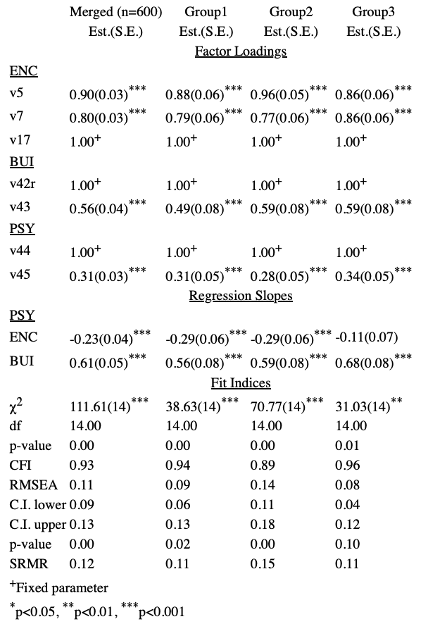
```{r create Table to compare three groups, warning = F, message = F}
estimator <- "ML"
# produce merged fit (200+200+200=600)
merged_fit <- sem(sem_multiGroup_model,
data = sim_multiGroupData_lavaan,
estimator = estimator,
std.lv = TRUE,
std.ov = TRUE,
group = NULL, # no grouping variable (e.g., gender, control/intervention,...)
cluster = NULL # no clustering variable (e.g., country)
# missing = "fiml.x" # full information maximum likelihood approach
)
# fit each group separately
group1_fit <- sem(sem_multiGroup_model,
data = sim_multiGroupData_lavaan[which(sim_multiGroupData_lavaan$group==1), ],
estimator = estimator,
std.lv = TRUE,
std.ov = TRUE,
group = NULL, # no grouping variable (e.g., gender, control/intervention,...)
cluster = NULL # no clustering variable (e.g., country)
# missing = "fiml.x" # full information maximum likelihood approach
)
group2_fit <- sem(sem_multiGroup_model,
data = sim_multiGroupData_lavaan[which(sim_multiGroupData_lavaan$group==2), ],
estimator = estimator,
std.lv = TRUE,
std.ov = TRUE,
group = NULL, # no grouping variable (e.g., gender, control/intervention,...)
cluster = NULL # no clustering variable (e.g., country)
# missing = "fiml.x" # full information maximum likelihood approach
)
group3_fit <- sem(sem_multiGroup_model,
data = sim_multiGroupData_lavaan[which(sim_multiGroupData_lavaan$group==3), ],
estimator = estimator,
std.lv = TRUE,
std.ov = TRUE,
group = NULL, # no grouping variable (e.g., gender, control/intervention,...)
cluster = NULL # no clustering variable (e.g., country)
# missing = "fiml.x" # full information maximum likelihood approach
)
library(semTable)
semTable(list(
"Merged (n=600)" = merged_fit,
"Group1" = group1_fit,
"Group2" = group2_fit,
"Group3" = group3_fit),
paramSets = c(
"loadings",
"slopes",
# "intercepts",
# "residualvariances",
# "residualcovariances",
# "latentmeans",
# "latentvariances",
# "latentcovariances",
# "thresholds",
# "constructed",
"fits"
),
paramSetLabels = c(
"loadings" = "Factor Loadings",
"slopes" = "Regression Slopes",
"intercepts" = "Intercepts",
"means"= "Means",
"residualvariances" = "Residual Variances",
"residualcovariances" = "Residual Covariances",
"variances" = "Variances",
"latentvariances" = "Latent Variances",
"latentcovariances" = "Latent Covariances",
"latentmeans" = "Latent Intercepts",
"thresholds" = "Thresholds",
"constructed" = "Constructed",
"fits" = "Fit Indices"
),
columns = c(
# "est",
# "se",
# "z",
# "p",
# "rsquare",
# "estse",
# "eststars",
"estsestars"
),
# columns = list("fit1" = c("est", "se"), "fit2" = c("estse", "p"))
columnLabels = c(
est = "Est.",
se = "S.E.",
z = "z",
p = "p",
rsquare = "R^2",
estse = "Est.(S.E.)",
eststars = "Est.",
estsestars = "Est.(S.E.)"
),
fits = c(
# "npar",
# "fmin",
"chisq",
"df",
"pvalue",
# "baseline.chisq",
# "baseline.df",
# "baseline.pvalue",
"cfi", # "ML"
# "cfi.scaled", # NOTE: WLSMV "appropriate" scaled fits
# "tli",
# "nnfi",
# "rfi",
# "nfi",
# "pnfi",
# "ifi",
# "rni",
# "logl",
# "unrestricted.logl",
# "aic",
# "bic",
# "ntotal",
# "bic2",
"rmsea", # good for "ML"
"rmsea.ci.lower",
"rmsea.ci.upper",
"rmsea.pvalue",
# "rmsea.scaled", # "WLSMV"
# "rmsea.ci.lower.scaled",
# "rmsea.ci.upper.scaled",
# "rmsea.pvalue.scaled",
# "rmr",
# "rmr_nomean",
"srmr"
# "srmr_bentler",
# "srmr_bentler_nomean",
# "srmr_bollen",
# "srmr_bollen_nomean",
# "srmr_mplus",
# "srmr_mplus_nomean",
# "cn_05",
# "cn_01",
# "gfi",
# "agfi",
# "pgfi",
# "mfi",
# "ecvi"
),
fitLabels = c(
df = "df",
pvalue = "p-value",
cfi = "CFI",
# cfi.scaled = "CFI", # NOTE: WLSMV "appropriate" scaled fits
# aic = "AIC",
# bic = "BIC",
rmsea = "RMSEA",
rmsea.ci.lower = "C.I. lower",
rmsea.ci.upper = "C.I. upper",
rmsea.pvalue = "p-value",
# rmsea.scaled = "RMSEA", # NOTE: WLSMV
# rmsea.ci.lower.scaled = " C.I. lower",
# rmsea.ci.upper.scaled = " C.I. upper",
# rmsea.pvalue.scaled = " p-value",
srmr = "SRMR"
),
file="Table_X_SEM_results", # where to save the table?
print.results = F,
type="html",
# type="latex",
longtable = TRUE,
table.float = TRUE,
caption ="XXX") #,
# label ="tab : fit5t2")
```
Show the table above:
```{r EXTRA plot SEM model, warning = F, message = F}
# library(lavaan)
# library(semPlot)
# library(semptools)
#
# dataEstFinIta <- read.table("dataEstFinIta.txt", header=TRUE, sep= "\t")
#
# # ------------
# # create model
#
# dfb_m4 <- '
# # Measurement model (factors)
# WorkTasks =~ wle2.1 + wle2.2 + wle4.2 + wle4.3 # Challenging and developing work tasks
# Resources =~ wle3.1 + wle3.2 + wle3.3 # Resources to help learning
# Recognition =~ wle6.1 + wle6.2 + wle7.1 # Recognition as expert and learner
# Congruence =~ wle8.1 + wle8.2 # Congruence with organizational goals
#
# # Regressions
# WorkTasks + Resources + Recognition ~ Congruence
#
#
# # Covariances
# WorkTasks ~~ Resources
# WorkTasks ~~ Recognition
# Recognition ~~ Resources
#
# '
#
# # ---
# # fit
#
# dfb_m4.fit <- sem(dfb_m4,
# data = dataEstFinIta,
# estimator = "WLSMV"
# )
#
#
# # ------------
# # prepare plot
#
# dfb_m4.fit.p1.std <- semPaths(dfb_m4.fit, # std estimates
# whatLabels="std", # optionally "est"
# sizeMan = 5,
# node.width = 1,
# edge.label.cex = .75,
# # style = "ram",
# intercepts=FALSE,
# mar = c(5, 5, 5, 5)) # ,
# # layout = layout)
#
#
# # -----------
# # define plot
#
# indicator_order <- c(
# "wle3.1", "wle3.2", "wle3.3",
# "wle2.1", "wle2.2", "wle4.2", "wle4.3",
# # "wle1.2", "wle1.3",
# "wle6.1", "wle6.2", "wle7.1",
# "wle8.1", "wle8.2")
#
# indicator_factor <- c( "Resources", "Resources", "Resources",
# "WorkTasks", "WorkTasks", "WorkTasks", "WorkTasks",
# # "Participation", "Participation",
# "Recognition", "Recognition", "Recognition",
# "Congruence", "Congruence")
#
# factor_layout <- layout_matrix(Resources = c(1, 3),
# WorkTasks = c(5, 3),
# Recognition = c(9, 3),
# Congruence = c(5, 1))
#
# factor_point_to <- layout_matrix(right = c(1, 3),
# right = c(5, 3),
# right = c(9, 3),
# left = c(5, 1))
#
# indicator_push <- c(Resources = 1.2,
# WorkTasks = 1.2,
# # Participation = 1,
# Recognition = 1.2,
# Congruence = 1.2)
#
# indicator_spread <- c(Resources = 4,
# WorkTasks = 5,
# # Participation = 4.5,
# Recognition = 4,
# Congruence = 3)
#
# loading_position <- c(Resources = .5,
# WorkTasks = .5,
# # Participation = .5,
# Recognition = .5,
# Congruence = .5)
#
# dfb_m4.fit.p2 <- set_sem_layout(dfb_m4.fit.p1.std, # standardized
# indicator_order = indicator_order,
# indicator_factor = indicator_factor,
# factor_layout = factor_layout,
# factor_point_to = factor_point_to,
# indicator_push = indicator_push,
# indicator_spread = indicator_spread,
# loading_position = loading_position) |>
# mark_sig(dfb_m4.fit) |> # show sig
# set_curve(c(
# "Resources ~~ WorkTasks" = -2,
# "WorkTasks ~~ Recognition" = -2,
# "Recognition ~~ Resources" = -4.9)
# )
#
#
#
#
# rotate_residuals <- c(Resources = 0,
# Congruence = 0,
# WorkTasks = -140,
# Recognition = -180)
#
# dfb_m4.fit.p2 <- rotate_resid(dfb_m4.fit.p2, rotate_residuals)
#
# plot(dfb_m4.fit.p2)
```
## References
Beaujean, A. A. (2014). *Latent Variable Modeling Using R. A Step-by-Step Guide.* Routledge.
Ferrer, E., Bolker, S. M., & Grimm, K. J. (2019). *Longitudinal Multivariate Psychology.* Routledge.